Let’s begin by first answering what is OCV or On-Chip-Variation during Static Timing Analysis (STA) in an ASIC Physical Design cycle?
On-Chip Variation (OCV) in Static Timing Analysis (STA) accounts for the variability of process parameters, voltages, and temperatures (PVT) within a single chip. Unlike global variations, which assume uniform PVT conditions across the entire chip, OCV recognizes that different parts of a chip can experience variations in these parameters simultaneously. OCV is considered for a single PVT.
On-Chip Variation (OCV) refers to manufacturing and environmental variations across a chip that cause differences in delay and slew rates of identical cells/nets. These variations arise from:
- Process: Transistor threshold voltage (Vth), oxide thickness variations.
- Voltage (IR Drop): Local power supply fluctuations.
- Temperature (Thermal Gradients): Hotspots vs. cooler regions.
CLOCK Uncertainty: CLOCK uncertainty includes components of skew variance, jitter and OCV variations.
Jitter : Is termed as the deviation of clock edge from its ideal location.
Now, we will try to understand how to correctly account for OCV during STA.
To account for On-Chip Variation (OCV) during Static Timing Analysis (STA), specific techniques and methodologies are employed to model and analyze the timing impacts of variability across different parts of the chip.
OCV is modeled in STA to ensure timing robustness by accounting for worst-case delays. Key concepts on how OCV is handled during STA:
1. Apply Derating Factors
- OCV Derates are scaling factors applied to delays and constraints to model timing variability between different parts of the chip.
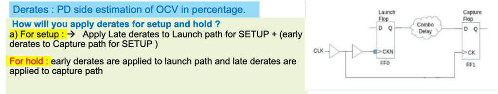
- Separate derating factors are applied for setup analysis (slower paths) and hold analysis (faster paths) to model worst-case scenarios:
- Setup Analysis: Increase the delays on data paths and decrease clock path delays to mimic worst-case scenarios for setup violations.
- Hold Analysis: Decrease the delays on data paths and increase clock path delays to mimic worst-case scenarios for hold violations.
- These derating factors can be specified as percentages (e.g., ±10%) and are provided in the timing library or manually defined.
2. Perform Multi-Corner, Multi-Mode (MCMM) Analysis
- OCV is analyzed across various process corners (e.g., slow-slow, fast-fast, typical-typical), voltage levels, and temperatures to ensure robustness across all conditions.
- Each mode and corner is analyzed with OCV applied.
3. Advanced OCV Models
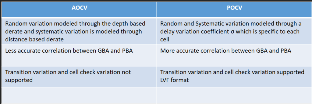
- AOCV (Advanced OCV):
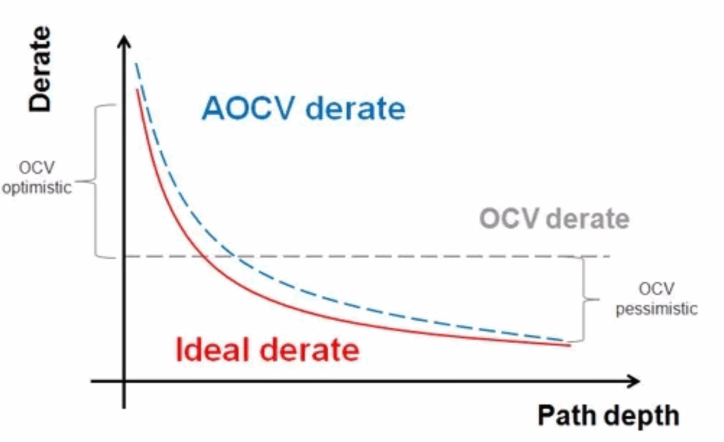
- Models OCV more realistically by considering the path depth and path location in the design.
- Long paths with more stages are less impacted by OCV due to averaging effects, while short paths are more affected.
- AOCV uses lookup tables to apply stage-aware derates.
- POCV (Parametric OCV):
- Extends AOCV by using statistical models to compute delays based on variations and probabilities.
- Provides a more accurate and less pessimistic timing analysis compared to static OCV or AOCV.
POCV (Parametric On-Chip Variation) settings are used in Static Timing Analysis (STA) to model timing variations more accurately by incorporating statistical variation into path delays, as opposed to using fixed derates like in traditional OCV or AOCV approaches.
POCV provides more realistic and less pessimistic results by modeling the probability distribution of delay variation.
set_pocv_stddev 0.05 ; # 5% standard deviation ns for each segment of a timing path.
4. Setup and Hold Timing Checks
- STA tools (e.g., Synopsys PrimeTime, Cadence Tempus) apply OCV-aware derates while performing setup and hold timing checks.
- Timing reports explicitly include OCV-adjusted delays for clock and data paths.
5. Group-Specific OCV (GOCV)
- For regions of the chip that share similar characteristics (e.g., same clock domain or physical proximity), specific OCV factors can be applied, reducing over-pessimism.
6. Margin Adjustments
- Incorporate additional margins during clock tree synthesis (CTS) or placement/routing to account for variability.
- Use margins judiciously to avoid excessive pessimism that impacts design performance.
7. Tool-Specific Features
- Modern STA tools support OCV methodologies natively:
- Synopsys PrimeTime: Supports OCV, AOCV, and POCV.
- Cadence Tempus: Provides OCV-aware timing analysis and optimization.
- Mentor Graphics (Siemens) Timequest: Incorporates OCV analysis for FPGAs and ASICs.
OCV vs. Other Variation Models
| Model | Granularity | Pessimism | Use Case |
|---|---|---|---|
| Path-Based OCV | Global derating | High | Early design |
| AOCV | Path depth/location | Medium | Mid-stage signoff |
| POCV | Statistical (Gaussian) | Low | Advanced nodes (<7nm) |
| LOCV | Physical proximity | Medium-Low | Block-level STA |
Q: “How does OCV affect hold timing, and how would you fix it?”
“OCV increases hold margins by derating launch paths early (faster) and capture paths late (slower). Fixes include:
- Buffer insertion on short paths.
- LOCV-aware CTS to reduce skew variation.
- AOCV/POCV to reduce pessimism.”
Q: “Why is AOCV preferred over path-based OCV?”
“AOCV reduces pessimism by derating based on path depth and location. For example, a long path’s cells statistically average out variations, so derating decreases with depth, unlike fixed path-based OCV.”